

Introduction: In our previous blog post, we explored the concept of linear equations and their singularity or non-singularity. Now, let's dive into the fascinating world of visualizing linear equations as lines in the coordinate plane. By representing systems of linear equations as arrangements of lines, we can gain a clearer understanding of their solutions and properties. In this blog post, we will explore various examples of linear equations and their visual representations, examining how they intersect or align to determine singular or non-singular systems.
Visualizing Equations: a + b = 10
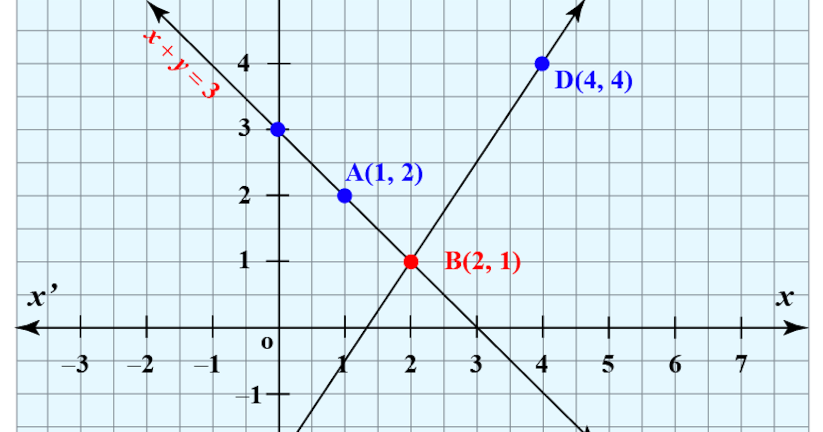
To begin, let's consider the equation a + b = 10, where 'a' represents the price of an apple, and 'b' represents the price of a banana. We can create a grid, with the horizontal axis representing 'a' and the vertical axis representing 'b.'
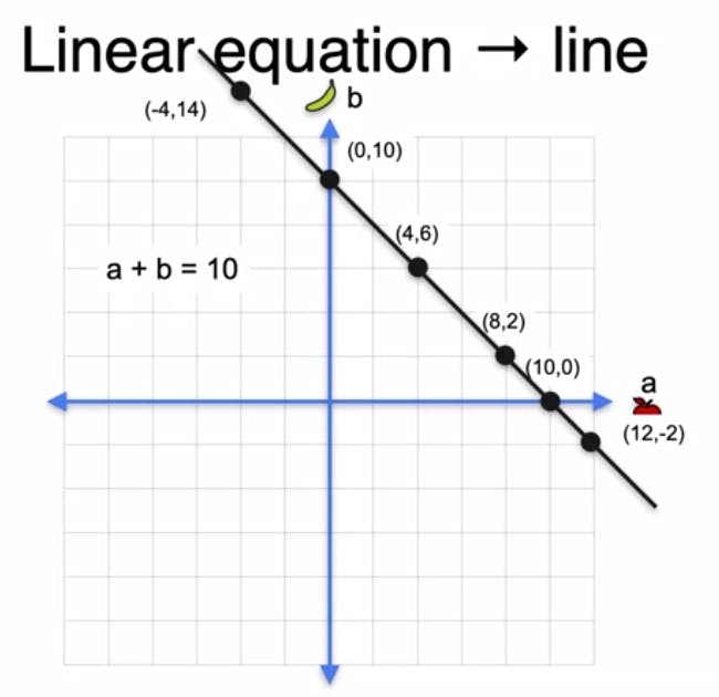
When we plot the solutions to this equation, we find that points like (10, 0), (0, 10), (4, 6), and (8, 2) lie on a line. These points represent pairs of numbers that add up to 10. Notably, we can have negative solutions, such as (-4, 14), which satisfy the equation. By connecting all these points, we obtain a line that encompasses every possible solution to the equation a + b = 10.
Visualizing Equations: a + 2b = 12
Now, let's examine the equation a + 2b = 12. Similar to the previous example, we plot points that satisfy this equation, including (0, 6), (12, 0), (8, 2), and even negative solutions like (-4, 8). These points form another line in the coordinate plane.

It is crucial to understand the notions of slope and y-intercept in a line. The slope represents the ratio of rise over run, indicating how the line moves in relation to the horizontal and vertical axes. In the first line, the slope is -1, meaning that for every unit we move to the right, the line moves one unit down. The y-intercept of this line is 10, as it intersects the vertical y-axis at that height. Similarly, the second line has a slope of -1/2 and a y-intercept of 6.
Visualizing Systems of Equations: Now, let's consider a system of two equations: a + b = 10 and a + 2b = 12. We visualize this system by plotting the two lines corresponding to these equations in the same coordinate plane.
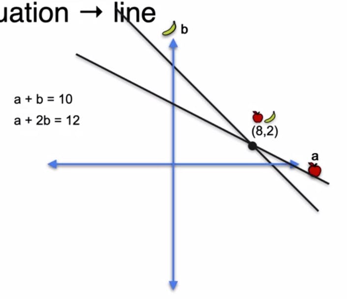
Remarkably, the two lines intersect at a unique point: (8, 2). This point represents the solution to the system of equations. Geometrically, the intersection of the lines captures the algebraic solution we obtained earlier. In this case, the system is non-singular because it has a unique solution.
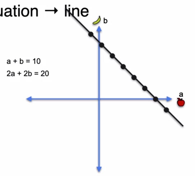
In contrast, when we examine the system a + b = 10 and 2a + 2b = 20, we observe that the two lines coincide. These lines overlap each other entirely, indicating that every point on the line satisfies both equations. Thus, the system has infinitely many solutions and is singular because the second equation does not bring any new information.

Lastly, let's analyze the system a + b = 10 and 2a + 2b = 24. When we plot the line associated with the equation 2a + 2b = 24, we notice that it runs parallel to the first line but is translated upward by two units. As the two lines are parallel, they never intersect, resulting in no shared solutions. Hence, this system is contradictory and singular.

To summarize our findings, we explored three systems of equations and their visual representations:
The first system, with equations a + b = 10 and a + 2b = 12, has a unique solution and is non-singular.
The second system, with equations a + b = 10 and 2a + 2b = 20, has infinitely many solutions and is singular.
The third system, with equations a + b = 10 and 2a + 2b = 24, has no solutions and is contradictory and singular.
In conclusion, visualizing linear equations as lines in the coordinate plane offers valuable insights into their solutions and properties. By examining the intersections, overlapping, or parallel nature of these lines, we can determine the singularity or non-singularity of systems of equations.

To simplify the concepts of singularity and non-singularity, the constants in the systems of equations are considered. By setting all constants to 0, the plots of the systems are transformed. The new systems always pass through the origin (0,0) since it becomes the solution.
System 1 remains a pair of intersecting lines, indicating a unique solution and non-singularity. System 2, with parallel lines, still has infinitely many solutions, maintaining its singularity. However, system 3, which initially had non-intersecting parallel lines, now becomes a pair of identical lines, resulting in infinitely many solutions instead of none. Although it changed from contradictory to redundant, it remains singular. The conclusion is that the constants in the system do not determine singularity or non-singularity.
Linear Dependence and Independence
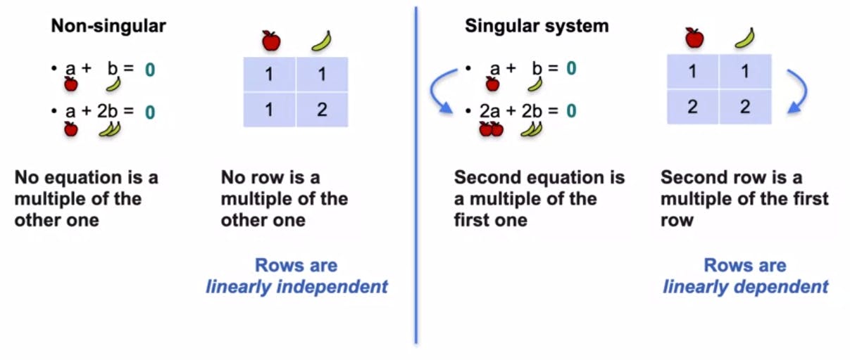
Linear dependence refers to a situation where one equation or row in a system or matrix can be expressed as a multiple of another equation or row. In other words, the information carried by one equation is redundant because it can be obtained from another equation. This leads to a singular system or matrix.
Linear independence, on the other hand, occurs when no equation or row in a system or matrix can be expressed as a multiple of another equation or row. Each equation or row in a non-singular system or matrix provides unique and independent information.
The same concepts of linear dependence and independence can also be applied to columns in a matrix. Determining whether a matrix is singular or non-singular relies on analyzing the linear dependency between its rows and columns.
The determinant

The determinant is a quick formula that determines whether a matrix is singular or non-singular. It returns a value of 0 for a singular matrix and a non-zero value for a non-singular matrix. A matrix is singular if its rows are linearly dependent, meaning that one row can be obtained by multiplying another row by a constant. The determinant of a matrix with entries a, b, c, and d is given by ad - bc. If the determinant is 0, the matrix is singular; if it is non-zero, the matrix is non-singular.